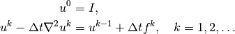
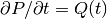
The examples in the section Fundamentals illustrate that solving linear, stationary PDE problems with the aid of FEniCS is easy and requires little programming. That is, FEniCS automates the spatial discretization by the finite element method. The solution of nonlinear problems, as we showed in the section Nonlinear Problems, can also be automated (cf. The section Solving the Nonlinear Variational Problem Directly), but many scientists will prefer to code the solution strategy of the nonlinear problem themselves and experiment with various combinations of strategies in difficult problems. Time-dependent problems are somewhat similar in this respect: we have to add a time discretization scheme, which is often quite simple, making it natural to explicitly code the details of the scheme so that the programmer has full control. We shall explain how easily this is accomplished through examples.
Our time-dependent model problem for teaching purposes is naturally the simplest extension of the Poisson problem into the time domain, i.e., the diffusion problem
Here,  varies with space and time, e.g.,
  if the spatial
domain
if the spatial
domain  is two-dimensional. The source function
  and the
boundary values
and the
boundary values  may also vary with space and time.
The initial condition
may also vary with space and time.
The initial condition  is a function of space only.
A straightforward approach to solving time-dependent PDEs by the finite element method is to first discretize the time derivative by a finite difference approximation, which yields a recursive set of stationary problems, and then turn each stationary problem into a variational formulation.
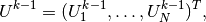
Let superscript  denote
a quantity at time
denote
a quantity at time  ,
where is an integer counting time levels. For example,
,
where is an integer counting time levels. For example,  means
at time level .
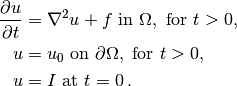
A finite difference discretization in time first consists in
sampling the PDE at some time level, say :
means
at time level .
A finite difference discretization in time first consists in
sampling the PDE at some time level, say :
(1)
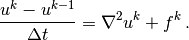
The time-derivative can be approximated by a finite difference. For simplicity and stability reasons we choose a simple backward difference:
(2)
where  is the time discretization parameter.
Inserting this approximation in the PDE yields
is the time discretization parameter.
Inserting this approximation in the PDE yields
(3)
This is our time-discrete version of the diffusion PDE
problem. Reordering the last equation
so that appears
on the left-hand side only,
yields
a recursive set of
spatial (stationary) problems for (assuming  is known from
computations at the previous time level):
is known from
computations at the previous time level):
Given , we can solve for  ,
,  ,
,  , and so on.
We use a finite element method
to solve the
time-discrete equations which still have spatial differential operators.
This requires turning the equations into weak forms.
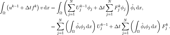
As usual, we multiply by a test function  and integrate
second-derivatives by parts. Introducing the symbol for
(which is natural in the program too), the resulting weak
form can be conveniently written in the standard notation:
and integrate
second-derivatives by parts. Introducing the symbol for
(which is natural in the program too), the resulting weak
form can be conveniently written in the standard notation:
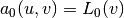 for the initial step
and
for the initial step
and 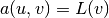 for a general step, where
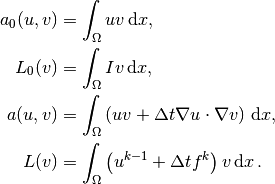
The continuous variational problem is to find
 such that
  holds for all
  ,
and then find
,
and then find  such that
  for all ,
 .
.
Approximate solutions in space
are found by
restricting the functional spaces  and
and  to finite-dimensional spaces,
exactly as we have done in the Poisson problems.
We shall use the symbol for the finite element
approximation at time . In case we need to distinguish this
space-time discrete approximation from the exact solution of
the continuous diffusion problem, we use
to finite-dimensional spaces,
exactly as we have done in the Poisson problems.
We shall use the symbol for the finite element
approximation at time . In case we need to distinguish this
space-time discrete approximation from the exact solution of
the continuous diffusion problem, we use  for the latter.
By we mean, from now on, the finite element approximation
of the solution at time
for the latter.
By we mean, from now on, the finite element approximation
of the solution at time  .
.
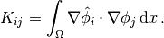
Note that the forms  and
and  are identical to the forms
met in the section Computing Derivatives, except that the test and trial
functions are now
scalar fields and not vector fields.
Instead of solving
an equation for
by a finite
element method, i.e., projecting onto via
the problem , we could simply interpolate from
. That is, if
are identical to the forms
met in the section Computing Derivatives, except that the test and trial
functions are now
scalar fields and not vector fields.
Instead of solving
an equation for
by a finite
element method, i.e., projecting onto via
the problem , we could simply interpolate from
. That is, if  , we
simply set
, we
simply set  , where
  are the coordinates of
node number
are the coordinates of
node number  . We refer to these two strategies as computing
the initial condition by either projecting or interpolating .
Both operations are easy to compute through one statement, using either
the project or interpolate function.
. We refer to these two strategies as computing
the initial condition by either projecting or interpolating .
Both operations are easy to compute through one statement, using either
the project or interpolate function.
Our program needs to perform the time stepping explicitly, but can
rely on FEniCS to easily compute , ,  , and
, and  , and solve
the linear systems for the unknowns. We realize that does not
depend on time, which means that its associated matrix also will be
time independent. Therefore, it is wise to explicitly create matrices
and vectors as in the section A Linear Algebra Formulation. The matrix
, and solve
the linear systems for the unknowns. We realize that does not
depend on time, which means that its associated matrix also will be
time independent. Therefore, it is wise to explicitly create matrices
and vectors as in the section A Linear Algebra Formulation. The matrix  arising from can be computed prior to the time stepping, so that
we only need to compute the right-hand side
arising from can be computed prior to the time stepping, so that
we only need to compute the right-hand side  , corresponding to ,
in each pass in the time loop. Let us express the solution procedure
in algorithmic form, writing for the unknown spatial function at
the new time level () and
, corresponding to ,
in each pass in the time loop. Let us express the solution procedure
in algorithmic form, writing for the unknown spatial function at
the new time level () and  for the spatial solution at one
earlier time level ():
for the spatial solution at one
earlier time level ():
- define Dirichlet boundary condition (
- if
- define
- assemble matrix
from
- solve
and store
in
- else: (interpolation)
- let
- define
- assemble matrix
- set some stopping time
- while
- assemble vector
- apply essential boundary conditions
- solve
for
(be ready for next step)
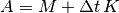
Before starting the coding, we shall construct a problem where it is easy to determine if the calculations are correct. The simple backward time difference is exact for linear functions, so we decide to have a linear variation in time. Combining a second-degree polynomial in space with a linear term in time,
(4)
yields a function whose computed values at the nodes may be exact,
regardless of the size of the elements and , as long as the
mesh is uniformly partitioned.
We realize by inserting the simple solution in the PDE problem
that must be given as
(?) and that  and
and  .
.
A new programming issue is how to deal with functions that vary in
space and time, such as the the boundary condition
.
A natural solution is
to apply an Expression object with time  as a parameter,
in addition to the parameters
as a parameter,
in addition to the parameters  and
and  (see
the section Solving a Real Physical Problem for Expression
objects with parameters):
(see
the section Solving a Real Physical Problem for Expression
objects with parameters):
alpha = 3; beta = 1.2
u0 = Expression('1 + x[0]*x[0] + alpha*x[1]*x[1] + beta*t',
                alpha=alpha, beta=beta, t=0)
The time parameter can later be updated by assigning values to u0.t.
Given a mesh and an associated function space V, we
can specify the function as
alpha = 3; beta = 1.2
u0 = Expression('1 + x[0]*x[0] + alpha*x[1]*x[1] + beta*t',
                {'alpha': alpha, 'beta': beta})
u0.t = 0
This function expression has the components of x as independent variables, while alpha, beta, and t are parameters. The parameters can either be set through a dictionary at construction time, as demonstrated for alpha and beta, or anytime through attributes in the function object, as shown for the t parameter.
The essential boundary conditions, along the whole boundary in this case, are set in the usual way,
def boundary(x, on_boundary):  # define the Dirichlet boundary
    return on_boundary

bc = DirichletBC(V, u0, boundary)
We shall use u for the unknown at the new time level and
u_1 for at the previous time level. The initial value of
u_1, implied by the initial condition on , can be computed
by either projecting or interpolating .
The  function is available in the program through
u0,
as long as u0.t is zero.
We can then do
function is available in the program through
u0,
as long as u0.t is zero.
We can then do
u_1 = interpolate(u0, V)
# or
u_1 = project(u0, V)
Note that we could, as an equivalent alternative to using project, define
and as we did in the section Computing Derivatives and form
the associated variational problem.
To actually recover the exact solution
to machine precision,
it is important not to compute the discrete initial condition by
projecting , but by interpolating so that the nodal values are
exact at  (projection results in approximative values at the nodes).
The definition of and goes as follows:
dt = 0.3      # time step

u = TrialFunction(V)
v = TestFunction(V)
f = Constant(beta - 2 - 2*alpha)

a = u*v*dx + dt*inner(grad(u), grad(v))*dx
L = (u_1 + dt*f)*v*dx

A = assemble(a)   # assemble only once, before the time stepping
Finally, we perform the time stepping in a loop:
u = Function(V)   # the unknown at a new time level
T = 2             # total simulation time
t = dt

while t <= T:
    b = assemble(L)
    u0.t = t
    bc.apply(A, b)
    solve(A, u.vector(), b)

    t += dt
    u_1.assign(u)
Observe that u0.t must be updated before the bc.apply statement, to enforce computation of Dirichlet conditions at the current time level.
The time loop above does not contain any comparison of the numerical and the exact solution, which we must include in order to verify the implementation. As in many previous examples, we compute the difference between the array of nodal values of u and the array of the interpolated exact solution. The following code is to be included inside the loop, after u is found:
u_e = interpolate(u0, V)
maxdiff = numpy.abs(u_e.vector().array()-u.vector().array()).max()
print 'Max error, t=%.2f: %-10.3f' % (t, maxdiff)
The right-hand side vector b must obviously be recomputed at each time level. With the construction b = assemble(L), a new vector for b is allocated in memory in every pass of the time loop. It would be much more memory friendly to reuse the storage of the b we already have. This is easily accomplished by
b = assemble(L, tensor=b)
That is, we send in our previous b, which is then filled with new values and returned from assemble. Now there will be only a single memory allocation of the right-hand side vector. Before the time loop we set b = None such that b is defined in the first call to assemble.
The complete program code for this time-dependent case is stored in the file d1_d2D.py in the directory transient/diffusion.
The purpose of this section is to present a technique for speeding
up FEniCS simulators for time-dependent problems where it is
possible to perform all assembly operations prior to the time loop.
There are two costly operations in the time loop: assembly of the
right-hand side and solution of the linear system via the
solve call. The assembly process involves work proportional to
the number of degrees of freedom  , while the solve operation
has a work estimate of
, while the solve operation
has a work estimate of  , for some
  . As
. As
 , the solve operation will dominate for
  ,
but for the values of typically used on smaller computers, the
assembly step may still
represent a considerable part of the total work at each
time level. Avoiding repeated assembly can therefore contribute to a
significant speed-up of a finite element code in time-dependent problems.
,
but for the values of typically used on smaller computers, the
assembly step may still
represent a considerable part of the total work at each
time level. Avoiding repeated assembly can therefore contribute to a
significant speed-up of a finite element code in time-dependent problems.
To see how repeated assembly can be avoided, we look at the  form,
which in general varies with
time through ,
form,
which in general varies with
time through ,  , and possibly also with
if the time step is adjusted during the simulation.
The technique for avoiding repeated assembly consists in
expanding the finite element functions in sums over the basis functions
, and possibly also with
if the time step is adjusted during the simulation.
The technique for avoiding repeated assembly consists in
expanding the finite element functions in sums over the basis functions
 , as explained
in the section A Linear Algebra Formulation, to identify matrix-vector
products that build up the complete system. We have
, as explained
in the section A Linear Algebra Formulation, to identify matrix-vector
products that build up the complete system. We have
 , and we can expand as
 . Inserting these expressions in
and using
. Inserting these expressions in
and using
 result in
Introducing 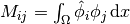 , we see that
the last expression can be written
, we see that
the last expression can be written
which is nothing but two matrix-vector products,
if is the matrix with entries  and
and
and
We have immediate access to  in the program since that is the vector
in the u_1 function. The
in the program since that is the vector
in the u_1 function. The  vector can easily be
computed by interpolating the prescribed function (at each time level if
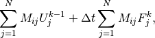
varies with time). Given , , and , the right-hand side
can be calculated as
vector can easily be
computed by interpolating the prescribed function (at each time level if
varies with time). Given , , and , the right-hand side
can be calculated as

That is, no assembly is necessary to compute .
The coefficient matrix can also be split into two terms.
We insert and 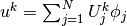 in
the relevant equations to get
in
the relevant equations to get
which can be written as a sum of matrix-vector products,

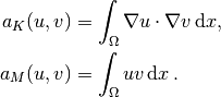
if we identify the matrix with entries as above and
the matrix  with entries
The matrix is often called the “mass matrix” while “stiffness matrix”
is a common nickname for . The associated bilinear forms for these
matrices, as we need them for the assembly process in a FEniCS
program, become
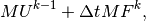
The linear system at each time level, written as  ,
can now be computed by first computing and , and then forming
,
can now be computed by first computing and , and then forming
 at , while is computed as
 at each time level.
The following modifications are needed in the d1_d2D.py program from the previous section in order to implement the new strategy of avoiding assembly at each time level:
- Define separate forms
and
- Assemble
to
- Compute
- Define
- Interpolate the formula for
- Compute
The relevant code segments become
# 1.
a_K = inner(grad(u), grad(v))*dx
a_M = u*v*dx
# 2. and 3.
M = assemble(a_M)
K = assemble(a_K)
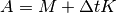
A = M + dt*K
# 4.
f = Expression('beta - 2 - 2*alpha', beta=beta, alpha=alpha)
# 5. and 6.
while t <= T:
f_k = interpolate(f, V)
F_k = f_k.vector()
b = M*u_1.vector() + dt*M*F_k
The complete program appears in the file d2_d2D.py.
With the basic programming techniques for time-dependent problems from
the sections Avoiding Assembly-Implementation (2)
we are ready to attack more physically realistic examples.
The next example concerns the question: How is the temperature in the
ground affected by day and night variations at the earth’s surface?
We consider some box-shaped domain in  dimensions with
coordinates
dimensions with
coordinates  (the problem is meaningful in 1D, 2D, and 3D).
At the top of the domain,
(the problem is meaningful in 1D, 2D, and 3D).
At the top of the domain,  , we have an oscillating
temperature
, we have an oscillating
temperature

where  is some reference temperature,
  is the amplitude of
the temperature variations at the surface, and
is the amplitude of
the temperature variations at the surface, and  is the frequency
of the temperature oscillations.
At all other boundaries we assume
that the temperature does not change anymore when we move away from
the boundary, i.e., the normal derivative is zero.
Initially, the temperature can be taken as everywhere.
The heat conductivity properties of the soil in the
ground may vary with space so
we introduce a variable coefficient
is the frequency
of the temperature oscillations.
At all other boundaries we assume
that the temperature does not change anymore when we move away from
the boundary, i.e., the normal derivative is zero.
Initially, the temperature can be taken as everywhere.
The heat conductivity properties of the soil in the
ground may vary with space so
we introduce a variable coefficient  reflecting this property.
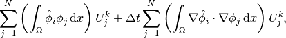
Figure Sketch of a (2D) problem involving heating and cooling of the ground due to an oscillating surface temperature shows a sketch of the
problem, with a small region where the heat conductivity is much lower.
reflecting this property.
Figure Sketch of a (2D) problem involving heating and cooling of the ground due to an oscillating surface temperature shows a sketch of the
problem, with a small region where the heat conductivity is much lower.
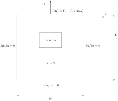
Sketch of a (2D) problem involving heating and cooling of the ground due to an oscillating surface temperature
The initial-boundary value problem for this problem reads
![\varrho c{\partial T\over\partial t} &= \nabla\cdot\left( \kappa\nabla T\right)\hbox{ in }\Omega\times (0,t_{\hbox{stop}}],\\
T &= T_0(t)\hbox{ on }\Gamma_0,\\
{\partial T\over\partial n} &= 0\hbox{ on }\partial\Omega\backslash\Gamma_0,\\
T &= T_R\hbox{ at }t =0\thinspace .](_images/math/7de14c412d02f82a0ad47ed9a7f8063ae233e424.png)
Here,  is the density of the soil,
  is the
heat capacity, is the thermal conductivity
(heat conduction coefficient)
in the soil, and
is the
heat capacity, is the thermal conductivity
(heat conduction coefficient)
in the soil, and  is the surface boundary .
We use a $theta$-scheme in time, i.e., the evolution equation
 is discretized as
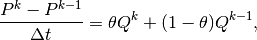
where ![\theta\in[0,1]](_images/math/72dd65603c76bb07232a019ad9e28777cd6eae35.png) is a weighting factor:
is a weighting factor:  corresponds
to the backward difference scheme,
corresponds
to the backward difference scheme,  to the Crank-Nicolson
scheme, and
to the Crank-Nicolson
scheme, and  to a forward difference scheme.
The $theta$-scheme applied to our PDE results in
to a forward difference scheme.
The $theta$-scheme applied to our PDE results in

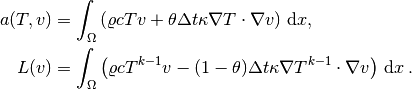
Bringing this time-discrete PDE into weak form follows the technique shown
many times earlier in this tutorial. In the standard notation
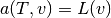 the weak form has
Observe that boundary integrals vanish because of the Neumann boundary conditions.
The size of a 3D box is taken as  , where
  is
the depth and
is
the depth and  is the width.
We give the degree of the basis functions at the command line, then ,
and then the divisions of the domain in the various directions.
To make a box, rectangle, or interval of arbitrary (not unit) size,
we have the DOLFIN classes Box, Rectangle, and
Interval at our disposal. The mesh and the function space
can be created by the following code:
is the width.
We give the degree of the basis functions at the command line, then ,
and then the divisions of the domain in the various directions.
To make a box, rectangle, or interval of arbitrary (not unit) size,
we have the DOLFIN classes Box, Rectangle, and
Interval at our disposal. The mesh and the function space
can be created by the following code:
degree = int(sys.argv[1])
D = float(sys.argv[2])
W = D/2.0
divisions = [int(arg) for arg in sys.argv[3:]]
d = len(divisions)  # no of space dimensions
if d == 1:
    mesh = Interval(divisions[0], -D, 0)
elif d == 2:
    mesh = Rectangle(-W/2, -D, W/2, 0, divisions[0], divisions[1])
elif d == 3:
    mesh = Box(-W/2, -W/2, -D, W/2, W/2, 0,
               divisions[0], divisions[1], divisions[2])
V = FunctionSpace(mesh, 'Lagrange', degree)
The Rectangle and Box objects are defined by the coordinates of the “minimum” and “maximum” corners.
Setting Dirichlet conditions at the upper boundary can be done by
T_R = 0; T_A = 1.0; omega = 2*pi

T_0 = Expression('T_R + T_A*sin(omega*t)',
                 T_R=T_R, T_A=T_A, omega=omega, t=0.0)

def surface(x, on_boundary):
    return on_boundary and abs(x[d-1]) < 1E-14

bc = DirichletBC(V, T_0, surface)
The function can be defined as a constant  inside
the particular rectangular area with a special soil composition, as
indicated in Figure Sketch of a (2D) problem involving heating and cooling of the ground due to an oscillating surface temperature. Outside
this area is a constant
inside
the particular rectangular area with a special soil composition, as
indicated in Figure Sketch of a (2D) problem involving heating and cooling of the ground due to an oscillating surface temperature. Outside
this area is a constant  .
The domain of the rectangular area is taken as
.
The domain of the rectangular area is taken as
![[-W/4, W/4]\times [-W/4, W/4]\times [-D/2, -D/2 + D/4]](_images/math/27e258f6381b7e54ee3178095168ecddc23c42c5.png)
in 3D, with ![[-W/4, W/4]\times [-D/2, -D/2 + D/4]](_images/math/ee353930fc1f00f02ea7f494e834c8e2825f9efe.png) in 2D and
in 2D and
![[-D/2, -D/2 + D/4]](_images/math/c07984601a803a1efcc0266944c8fa9d7f0255d1.png) in 1D.
Since we need some testing in the definition of the
in 1D.
Since we need some testing in the definition of the  function, the most straightforward approach is to define a subclass
of Expression, where we can use a full Python method instead of
just a C++ string formula for specifying a function.
The method that defines the function is called eval:
function, the most straightforward approach is to define a subclass
of Expression, where we can use a full Python method instead of
just a C++ string formula for specifying a function.
The method that defines the function is called eval:
class Kappa(Function):
    def eval(self, value, x):
        """x: spatial point, value[0]: function value."""
        d = len(x)  # no of space dimensions
        material = 0  # 0: outside, 1: inside
        if d == 1:
            if -D/2. < x[d-1] < -D/2. + D/4.:
                material = 1
        elif d == 2:
            if -D/2. < x[d-1] < -D/2. + D/4. and \
               -W/4. < x[0] < W/4.:
                material = 1
        elif d == 3:
            if -D/2. < x[d-1] < -D/2. + D/4. and \
               -W/4. < x[0] < W/4. and -W/4. < x[1] < W/4.:
                material = 1
        value[0] = kappa_0 if material == 0 else kappa_1
The eval method gives great flexibility in defining functions,
but a downside is that C++ calls up eval in Python for
each point x, which is a slow process, and the number of calls
is proportional to the number of nodes in the mesh.
Function expressions in terms of strings are compiled to efficient
C++ functions, being called from C++, so we should try to express functions
as string expressions if possible. (The eval method can also be
defined through C++ code, but this is much
more complicated and not covered here.)
Using inline if-tests in C++, we can make string expressions for
:
kappa_str = {}
kappa_str[1] = 'x[0] > -D/2 && x[0] < -D/2 + D/4 ? kappa_1 : kappa_0'
kappa_str[2] = 'x[0] > -W/4 && x[0] < W/4 '\
               '&& x[1] > -D/2 && x[1] < -D/2 + D/4 ? '\
               'kappa_1 : kappa_0'
kappa_str[3] = 'x[0] > -W/4 && x[0] < W/4 '\
               'x[1] > -W/4 && x[1] < W/4 '\
               '&& x[2] > -D/2 && x[2] < -D/2 + D/4 ?'\
               'kappa_1 : kappa_0'

kappa = Expression(kappa_str[d],
                   D=D, W=W, kappa_0=kappa_0, kappa_1=kappa_1)
Let T denote the unknown spatial temperature function at the current time level, and let T_1 be the corresponding function at one earlier time level. We are now ready to define the initial condition and the a and L forms of our problem:
T_prev = interpolate(Constant(T_R), V)

rho = 1
c = 1
period = 2*pi/omega
t_stop = 5*period
dt = period/20  # 20 time steps per period
theta = 1

T = TrialFunction(V)
v = TestFunction(V)
f = Constant(0)
a = rho*c*T*v*dx + theta*dt*kappa*\
    inner(grad(T), grad(v))*dx
L = (rho*c*T_prev*v + dt*f*v -
     (1-theta)*dt*kappa*inner(grad(T), grad(v)))*dx

A = assemble(a)
b = None  # variable used for memory savings in assemble calls
T = Function(V)   # unknown at the current time level
We could, alternatively, break a and L up in subexpressions and assemble a mass matrix and stiffness matrix, as exemplified in the section Avoiding Assembly, to avoid assembly of b at every time level. This modification is straightforward and left as an exercise. The speed-up can be significant in 3D problems.
The time loop is very similar to what we have displayed in the section Implementation (2):
T = Function(V)   # unknown at the current time level
t = dt
while t <= t_stop:
    b = assemble(L, tensor=b)
    T_0.t = t
    bc.apply(A, b)
    solve(A, T.vector(), b)
    # visualization statements
    t += dt
    T_prev.assign(T)
The complete code in sin_daD.py contains several statements related to visualization and animation of the solution, both as a finite element field (plot calls) and as a curve in the vertical direction. The code also plots the exact analytical solution,
which is valid when  .
.
Implementing this analytical solution as a Python function taking scalars and numpy arrays as arguments requires a word of caution. A straightforward function like
def T_exact(x):
    a = sqrt(omega*rho*c/(2*kappa_0))
    return T_R + T_A*exp(a*x)*sin(omega*t + a*x)
will not work and result in an error message from UFL. The reason is that the names exp and sin are those imported by the from dolfin import * statement, and these names come from UFL and are aimed at being used in variational forms. In the T_exact function where x may be a scalar or a numpy array, we therefore need to explicitly specify numpy.exp and numpy.sin:
def T_exact(x):
    a = sqrt(omega*rho*c/(2*kappa_0))
    return T_R + T_A*numpy.exp(a*x)*numpy.sin(omega*t + a*x)
The reader is encouraged to play around with the code and test out various parameter sets:
,
,
,
,
,
,
,
C,
C,
,
,
,
,
1/h
1/s,
m
- As above, but
and
Data set number 4 is relevant for real temperature variations in
the ground (not necessarily the large value of ),
while data set number 5
exaggerates the effect of a large heat conduction contrast so that
it becomes clearly visible in an animation.