
Now we shall address how to solve nonlinear PDEs in FEniCS. Our sample PDE for implementation is taken as a nonlinear Poisson equation:
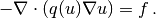
The coefficient  makes the equation nonlinear (unless
is constant in
makes the equation nonlinear (unless
is constant in  ).
).
To be able to easily verify our implementation,
we choose the domain, ,  , and the boundary
conditions such that we have
a simple, exact solution . Let
, and the boundary
conditions such that we have
a simple, exact solution . Let
 be the unit hypercube
 ![[0, 1]^d](_images/math/0ee1e007f47139a819af6241b0bdd8fee169e767.png) in
in  dimensions,
  ,
,  ,
,  for
for  ,
,  for
for  , and
, and  at all other boundaries
 and
and  ,
,  . The coordinates are now represented by
the symbols
. The coordinates are now represented by
the symbols  . The exact solution is then

We refer to the section Parameterizing the Number of Space Dimensions for details on formulating a PDE
problem in space dimensions.
The variational formulation of our model problem reads:
Find  such that
(1)
where
(2)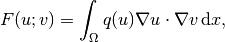
and
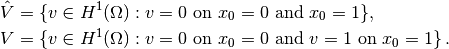
The discrete problem arises as usual by restricting  and
and  to a
pair of discrete spaces. As usual, we omit any subscript on discrete
spaces and simply say and are chosen finite dimensional
according to some mesh with some element type.
Similarly, we let be the discrete solution and use
to a
pair of discrete spaces. As usual, we omit any subscript on discrete
spaces and simply say and are chosen finite dimensional
according to some mesh with some element type.
Similarly, we let be the discrete solution and use  for
the exact solution if it becomes necessary to distinguish between the two.
for
the exact solution if it becomes necessary to distinguish between the two.
The discrete nonlinear problem is then wirtten as: find  such that
(3)
with  . Since
  is a nonlinear function
of , the variational statement gives rise to a system of
nonlinear algebraic equations.
[[[
FEniCS can be used in alternative ways for solving a nonlinear PDE
problem. We shall in the following subsections go through four
solution strategies:
is a nonlinear function
of , the variational statement gives rise to a system of
nonlinear algebraic equations.
[[[
FEniCS can be used in alternative ways for solving a nonlinear PDE
problem. We shall in the following subsections go through four
solution strategies:
- a simple Picard-type iteration,
- a Newton method at the algebraic level,
- a Newton method at the PDE level, and
- an automatic approach where FEniCS attacks the nonlinear variational problem directly.
The “black box” strategy 4 is definitely the simplest one from a programmer’s point of view, but the others give more manual control of the solution process for nonlinear equations (which also has some pedagogical advantages, especially for newcomers to nonlinear finite element problems).
Picard iteration is an easy way of handling nonlinear PDEs: we simply
use a known, previous solution in the nonlinear terms so that these
terms become linear in the unknown . The strategy is also known as
the method of successive substitutions.
For our particular problem,
we use a known, previous solution in the coefficient .
More precisely, given a solution  from iteration
  , we seek a
new (hopefully improved) solution
, we seek a
new (hopefully improved) solution  in iteration
  such
that solves the linear problem,
such
that solves the linear problem,
(4)
The iterations require an initial guess  .
The hope is that
.
The hope is that  as
as  , and that
is sufficiently close to the exact
solution of the discrete problem after just a few iterations.
, and that
is sufficiently close to the exact
solution of the discrete problem after just a few iterations.
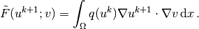
We can easily formulate a variational problem for from
the last equation.
Equivalently, we can approximate by  in
in
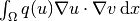 to obtain the same linear variational problem.
In both cases, the problem consists of seeking
to obtain the same linear variational problem.
In both cases, the problem consists of seeking
 such that
(5)
with
(6)
Since this is a linear problem in the unknown , we can equivalently
use the formulation
with
The iterations can be stopped when  , where
  is a small tolerance, say
  , or
when the number of iterations exceed some critical limit. The latter
case will pick up divergence of the method or unacceptable slow
convergence.
, or
when the number of iterations exceed some critical limit. The latter
case will pick up divergence of the method or unacceptable slow
convergence.
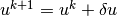
In the solution algorithm we only need to store and ,
called u_k and u in the code below.
The algorithm can then be expressed as follows:
def q(u):
    return (1+u)**m

# Define variational problem for Picard iteration
u = TrialFunction(V)
v = TestFunction(V)
u_k = interpolate(Constant(0.0), V)  # previous (known) u
a = inner(q(u_k)*grad(u), grad(v))*dx
f = Constant(0.0)
L = f*v*dx

# Picard iterations
u = Function(V)     # new unknown function
eps = 1.0           # error measure ||u-u_k||
tol = 1.0E-5        # tolerance
iter = 0            # iteration counter
maxiter = 25        # max no of iterations allowed
while eps > tol and iter < maxiter:
    iter += 1
    solve(a == L, u, bcs)
    diff = u.vector().array() - u_k.vector().array()
    eps = numpy.linalg.norm(diff, ord=numpy.Inf)
    print 'iter=%d: norm=%g' % (iter, eps)
    u_k.assign(u)   # update for next iteration
We need to define the previous solution in the iterations, u_k, as a finite element function so that u_k can be updated with u at the end of the loop. We may create the initial Function u_k by interpolating an Expression or a Constant to the same vector space as u lives in (V).
In the code above we demonstrate how to use
numpy functionality to compute the norm of
the difference between the two most recent solutions. Here we apply
the maximum norm ( norm) on the difference of the solution vectors
(ord=1 and ord=2 give the
norm) on the difference of the solution vectors
(ord=1 and ord=2 give the  and
and  vector
norms – other norms are possible for numpy arrays,
see pydoc numpy.linalg.norm).
vector
norms – other norms are possible for numpy arrays,
see pydoc numpy.linalg.norm).
The file picard_np.py contains the complete code for
this nonlinear Poisson problem.
The implementation is dimensional, with mesh
construction and setting of Dirichlet conditions as explained in
the section Parameterizing the Number of Space Dimensions.
For a  grid with
  we need 9 iterations for convergence
when the tolerance is .
we need 9 iterations for convergence
when the tolerance is .
After having discretized our nonlinear PDE problem, we may
use Newton’s method to solve the system of nonlinear algebraic equations.
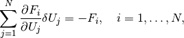
From the continuous variational problem,
the discrete version results in a
system of equations for the unknown parameters 
(7)
Newton’s method for the system 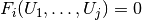 ,
,  can be formulated as
where ![\omega\in [0,1]](_images/math/c918e3e2e228f3ed67d74bcf2a5cda9c4aabfa48.png) is a relaxation parameter, and is
an iteration index. An initial guess must
be provided to start the algorithm.
is a relaxation parameter, and is
an iteration index. An initial guess must
be provided to start the algorithm.
The original Newton method has  , but in problems where it is
difficult to obtain convergence,
so-called under-relaxation with
, but in problems where it is
difficult to obtain convergence,
so-called under-relaxation with  may help. It means that
one takes a smaller step than what is suggested by Newton’s method.
may help. It means that
one takes a smaller step than what is suggested by Newton’s method.
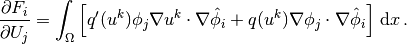
We need, in a program, to compute the Jacobian
matrix  and the right-hand side vector
  .
Our present problem has
.
Our present problem has  given by above.
The derivative becomes
given by above.
The derivative becomes
(8)
The following results were used to obtain the previous equation:
We can reformulate the Jacobian matrix
by introducing the short
notation 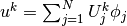 :
:
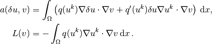
In order to make FEniCS compute this matrix, we need to formulate a corresponding variational problem. Looking at the linear system of equations in Newton’s method,
we can introduce  as a general test function replacing
  ,
and we can identify the unknown
,
and we can identify the unknown
 . From the linear system
we can now go “backwards” to construct the corresponding linear
discrete weak form to be solved in each Newton iteration:
. From the linear system
we can now go “backwards” to construct the corresponding linear
discrete weak form to be solved in each Newton iteration:
(9)
This variational form fits the standard notation
 with
with
Note the important feature in Newton’s method
that the
previous solution replaces
in the formulas when computing the matrix
and vector for the linear system in
each Newton iteration.
We now turn to the implementation.
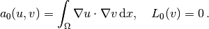
To obtain a good initial guess , we can solve a simplified, linear
problem, typically with  , which yields the standard Laplace
equation
, which yields the standard Laplace
equation  . The recipe for solving this problem
appears in the sections Variational Formulation,
Implementation (1), and Combining Dirichlet and Neumann Conditions.
The code for computing becomes as follows:
. The recipe for solving this problem
appears in the sections Variational Formulation,
Implementation (1), and Combining Dirichlet and Neumann Conditions.
The code for computing becomes as follows:
tol = 1E-14
def left_boundary(x, on_boundary):
    return on_boundary and abs(x[0]) < tol

def right_boundary(x, on_boundary):
    return on_boundary and abs(x[0]-1) < tol

Gamma_0 = DirichletBC(V, Constant(0.0), left_boundary)
Gamma_1 = DirichletBC(V, Constant(1.0), right_boundary)
bcs = [Gamma_0, Gamma_1]

# Define variational problem for initial guess (q(u)=1, i.e., m=0)
u = TrialFunction(V)
v = TestFunction(V)
a = inner(grad(u), grad(v))*dx
f = Constant(0.0)
L = f*v*dx
A, b = assemble_system(a, L, bcs)
u_k = Function(V)
U_k = u_k.vector()
solve(A, U_k, b)
Here, u_k denotes the solution function for the previous
iteration, so that the solution
after each Newton iteration is u = u_k + omega*du.
Initially, u_k is the initial guess we call in the mathematics.
The Dirichlet boundary conditions for  , in
the problem to be solved in each Newton
iteration, are somewhat different than the conditions for .
Assuming that fulfills the
Dirichlet conditions for , must be zero at the boundaries
where the Dirichlet conditions apply, in order for
, in
the problem to be solved in each Newton
iteration, are somewhat different than the conditions for .
Assuming that fulfills the
Dirichlet conditions for , must be zero at the boundaries
where the Dirichlet conditions apply, in order for 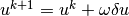 to fulfill
the right boundary values. We therefore define an additional list of
Dirichlet boundary conditions objects for :
to fulfill
the right boundary values. We therefore define an additional list of
Dirichlet boundary conditions objects for :
Gamma_0_du = DirichletBC(V, Constant(0), left_boundary)
Gamma_1_du = DirichletBC(V, Constant(0), right_boundary)
bcs_du = [Gamma_0_du, Gamma_1_du]
The nonlinear coefficient and its derivative must be defined before coding the weak form of the Newton system:
def q(u):
    return (1+u)**m

def Dq(u):
    return m*(1+u)**(m-1)

du = TrialFunction(V) # u = u_k + omega*du
a = inner(q(u_k)*grad(du), grad(v))*dx + \
    inner(Dq(u_k)*du*grad(u_k), grad(v))*dx
L = -inner(q(u_k)*grad(u_k), grad(v))*dx
The Newton iteration loop is very similar to the Picard iteration loop in the section Picard Iteration:
du = Function(V)
u  = Function(V)  # u = u_k + omega*du
omega = 1.0       # relaxation parameter
eps = 1.0
tol = 1.0E-5
iter = 0
maxiter = 25
while eps > tol and iter < maxiter:
    iter += 1
    A, b = assemble_system(a, L, bcs_du)
    solve(A, du.vector(), b)
    eps = numpy.linalg.norm(du.vector().array(), ord=numpy.Inf)
    print 'Norm:', eps
    u.vector()[:] = u_k.vector() + omega*du.vector()
    u_k.assign(u)
There are other ways of implementing the update of the solution as well:
u.assign(u_k)  # u = u_k
u.vector().axpy(omega, du.vector())

# or
u.vector()[:] += omega*du.vector()
The axpy(a, y) operation adds a scalar a times a Vector y to a Vector object. It is usually a fast operation calling up an optimized BLAS routine for the calculation.
Mesh construction for a $d$-dimensional problem with arbitrary degree of the Lagrange elements can be done as explained in the section Parameterizing the Number of Space Dimensions. The complete program appears in the file alg_newton_np.py.
Although Newton’s method in PDE problems is normally formulated at the linear algebra level, i.e., as a solution method for systems of nonlinear algebraic equations, we can also formulate the method at the PDE level. This approach yields a linearization of the PDEs before they are discretized. FEniCS users will probably find this technique simpler to apply than the more standard method in the section A Newton Method at the Algebraic Level.
Given an approximation to the solution field, , we seek a
perturbation so that
fulfills the nonlinear PDE.
However, the problem for is still nonlinear and nothing is
gained. The idea is therefore to assume that is sufficiently
small so that we can linearize the problem with respect to .
Inserting in the PDE,
linearizing the  term as

and dropping nonlinear terms in ,
we get

We may collect the terms with the unknown on the left-hand side,

The weak form of this PDE is derived by multiplying by a test function
and integrating over , integrating as usual
the second-order derivatives by parts:

The variational problem reads: find  such that
 for all
  , where
The function spaces and , being continuous or discrete,
are as in the
linear Poisson problem from the section Variational Formulation.
We must provide some initial guess, e.g., the solution of the
PDE with . The corresponding weak form 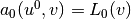 has
has
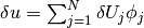
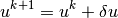
Thereafter, we enter a loop and solve
for and compute a new approximation
 . Note that is a correction, so if
satisfies the prescribed
Dirichlet conditions on some part
. Note that is a correction, so if
satisfies the prescribed
Dirichlet conditions on some part  of the boundary,
we must demand
of the boundary,
we must demand  on .
on .
Looking at the equations just derived,
we see that the variational form is the same as for the Newton method
at the algebraic level in the section A Newton Method at the Algebraic Level. Since Newton’s method at the
algebraic level required some “backward” construction of the
underlying weak forms, FEniCS users may prefer Newton’s method at the
PDE level, which this author finds more straightforward, although not so
commonly documented in the literature on numerical methods for PDEs.
There is seemingly no need for differentiations to derive a Jacobian
matrix, but a mathematically equivalent derivation is done when
nonlinear terms are linearized using the first two Taylor series terms
and when products in the perturbation are neglected.
The implementation is identical to the one in the section A Newton Method at the Algebraic Level and is found in the file pde_newton_np.py. The reader is encouraged to go through this code to be convinced that the present method actually ends up with the same program as needed for the Newton method at the linear algebra level in the section A Newton Method at the Algebraic Level.
The previous hand-calculations and manual implementation of Picard or Newton methods can be automated by tools in FEniCS. In a nutshell, one can just write
problem = NonlinearVariationalProblem(F, u, bcs, J)
solver  = NonlinearVariationalSolver(problem)
solver.solve()
where F corresponds to the nonlinear form  ,
u is the unknown Function object, bcs
represents the essential boundary conditions (in general a list of
DirichletBC objects), and
J is a variational form for the Jacobian of F.
,
u is the unknown Function object, bcs
represents the essential boundary conditions (in general a list of
DirichletBC objects), and
J is a variational form for the Jacobian of F.
Let us explain in detail how to use the built-in tools for nonlinear variational problems and their solution. The appropriate F form is straightforwardly defined as follows, assuming q(u) is coded as a Python function:
u_ = Function(V)     # most recently computed solution
v  = TestFunction(V)
F  = inner(q(u_)*grad(u_), grad(v))*dx
Note here that u_ is a Function (not a TrialFunction).
An alternative and perhaps more intuitive formula for is to
define directly in terms of
a trial function for and a test function for , and then
create the proper F by
u  = TrialFunction(V)
v  = TestFunction(V)
F  = inner(q(u)*grad(u), grad(v))*dx
u_ = Function(V)     # the most recently computed solution
F  = action(F, u_)
The latter statement is equivalent to  , where
  is
an existing finite element function representing the most recently
computed approximation to the solution.
(Note that and in the previous notation
correspond to and in the present
notation. We have changed notation to better align the mathematics with
the associated UFL code.)
is
an existing finite element function representing the most recently
computed approximation to the solution.
(Note that and in the previous notation
correspond to and in the present
notation. We have changed notation to better align the mathematics with
the associated UFL code.)
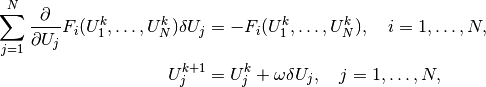
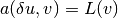
The derivative  (J) of (F) is formally the
Gateaux derivative
(J) of (F) is formally the
Gateaux derivative  of at
of at  in the direction of .
Technically, this Gateaux derivative is derived by computing
in the direction of .
Technically, this Gateaux derivative is derived by computing
(10)
The is now the trial function and is the previous
approximation to the solution .
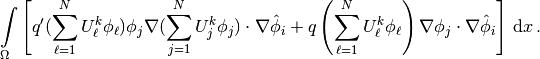
We start with
and obtain

which leads to
as  .
This last expression is the Gateaux derivative of . We may use or
.
This last expression is the Gateaux derivative of . We may use or
 for this derivative, the latter having the advantage
that we easily recognize the expression as a bilinear form. However, in
the forthcoming code examples J is used as variable name for
the Jacobian.
for this derivative, the latter having the advantage
that we easily recognize the expression as a bilinear form. However, in
the forthcoming code examples J is used as variable name for
the Jacobian.
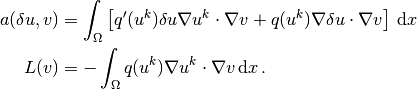
The specification of J goes as follows if du is the TrialFunction:
du = TrialFunction(V)
v  = TestFunction(V)
u_ = Function(V)      # the most recently computed solution
F  = inner(q(u_)*grad(u_), grad(v))*dx

J = inner(q(u_)*grad(du), grad(v))*dx + \
    inner(Dq(u_)*du*grad(u_), grad(v))*dx
The alternative specification of F, with u as TrialFunction, leads to
u  = TrialFunction(V)
v  = TestFunction(V)
u_ = Function(V)      # the most recently computed solution
F  = inner(q(u)*grad(u), grad(v))*dx
F  = action(F, u_)

J = inner(q(u_)*grad(u), grad(v))*dx + \
    inner(Dq(u_)*u*grad(u_), grad(v))*dx
The UFL language, used to specify weak forms, supports differentiation of forms. This feature facilitates automatic symbolic computation of the Jacobian J by calling the function derivative with F, the most recently computed solution (Function), and the unknown (TrialFunction) as parameters:
du = TrialFunction(V)
v  = TestFunction(V)
u_ = Function(V)      # the most recently computed solution
F  = inner(q(u_)*grad(u_), grad(v))*dx

J  = derivative(F, u_, du)  # Gateaux derivative in dir. of du
or
u  = TrialFunction(V)
v  = TestFunction(V)
u_ = Function(V)      # the most recently computed solution
F  = inner(q(u)*grad(u), grad(v))*dx
F  = action(F, u_)

J  = derivative(F, u_, u)   # Gateaux derivative in dir. of u
The derivative function is obviously very convenient in problems where differentiating F by hand implies lengthy calculations.
The preferred implementation of F and J, depending on whether du or u is the TrialFunction object, is a matter of personal taste. Derivation of the Gateaux derivative by hand, as shown above, is most naturally matched by an implementation where du is the TrialFunction, while use of automatic symbolic differentiation with the aid of the derivative function is most naturally matched by an implementation where u is the TrialFunction. We have implemented both approaches in two files: vp1_np.py with u as TrialFunction, and vp2_np.py with du as TrialFunction. The directory stationary/nonlinear_poisson contains both files. The first command-line argument determines if the Jacobian is to be automatically derived or computed from the hand-derived formula.
The following code defines the nonlinear variational problem and an associated solver based on Newton’s method. We here demonstrate how key parameters in Newton’s method can be set, as well as the choice of solver and preconditioner, and associated parameters, for the linear system occurring in the Newton iteration.
problem = NonlinearVariationalProblem(F, u_, bcs, J)
solver  = NonlinearVariationalSolver(problem)

prm = solver.parameters
prm['newton_solver']['absolute_tolerance'] = 1E-8
prm['newton_solver']['relative_tolerance'] = 1E-7
prm['newton_solver']['maximum_iterations'] = 25
prm['newton_solver']['relaxation_parameter'] = 1.0
if iterative_solver:
    prm['linear_solver'] = 'gmres'
    prm['preconditioner'] = 'ilu'
    prm['krylov_solver']['absolute_tolerance'] = 1E-9
    prm['krylov_solver']['relative_tolerance'] = 1E-7
    prm['krylov_solver']['maximum_iterations'] = 1000
    prm['krylov_solver']['gmres']['restart'] = 40
    prm['krylov_solver']['preconditioner']['ilu']['fill_level'] = 0
set_log_level(PROGRESS)

solver.solve()
A list of available parameters and their default values can as usual be printed by calling info(prm, True). The u_ we feed to the nonlinear variational problem object is filled with the solution by the call solver.solve().