
Solving PDEs in domains made up of different materials is a frequently encountered task. In FEniCS, these kind of problems are handled by defining subdomains inside the domain. The subdomains may represent the various materials. We can thereafter define material properties through functions, known in FEniCS as mesh functions, that are piecewise constant in each subdomain. A simple example with two materials (subdomains) in 2D will demonstrate the basic steps in the process. .. Later, a multi-material
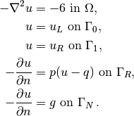
Suppose we want to solve
(1)
in a domain  consisting of two subdomains where
  takes on
a different value in each subdomain.
For simplicity, yet without loss of generality, we choose for the current
implementation
the domain
takes on
a different value in each subdomain.
For simplicity, yet without loss of generality, we choose for the current
implementation
the domain ![\Omega = [0,1]\times [0,1]](_images/math/5fa98371a9c614c641ca9e6393093bedbda39805.png) and divide it into two equal
subdomains,
and divide it into two equal
subdomains,
![\Omega_0 = [0, 1]\times [0,1/2],\quad
\Omega_1 = [0, 1]\times (1/2,1]\thinspace .](_images/math/eb4a679c7bea4121cf29bbba6d8ef6dbaded41b1.png)
We define  in
in  and
and  in
in  ,
where
,
where  and
and  are given constants.
As boundary conditions, we choose
are given constants.
As boundary conditions, we choose  at
at  ,
,  at
at  ,
and
,
and  at
at  and
and  .
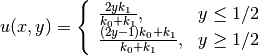
One can show that the exact solution is now given by
.
One can show that the exact solution is now given by
As long as the element boundaries coincide with the internal boundary
 , this piecewise linear solution should be exactly recovered
by Lagrange elements of any degree. We use this property to verify
the implementation.
, this piecewise linear solution should be exactly recovered
by Lagrange elements of any degree. We use this property to verify
the implementation.
Physically, the present problem may correspond to heat conduction, where
the heat conduction in is ten times more efficient than
in . An alternative interpretation is flow in porous media
with two geological layers, where the layers’ ability to transport
the fluid differs by a factor of 10.
The new functionality in this subsection regards how to
define the subdomains
and . For this purpose we need to
use subclasses of class SubDomain,
not only plain functions as we have used so far
for specifying boundaries. Consider the boundary function
def boundary(x, on_boundary):
    tol = 1E-14
    return on_boundary and abs(x[0]) < tol
for defining the boundary . Instead of using such a stand-alone
function, we can create an instance (or object)
of a subclass of SubDomain,
which implements the inside method as an alternative to the
boundary function:
class Boundary(SubDomain):
    def inside(self, x, on_boundary):
        tol = 1E-14
        return on_boundary and abs(x[0]) < tol

boundary = Boundary()
bc = DirichletBC(V, Constant(0), boundary)
A word about computer science terminology may be used here: The term instance means a Python object of a particular type (such as SubDomain, Function FunctionSpace, etc.). Many use instance and object as interchangeable terms. In other computer programming languages one may also use the term variable for the same thing. We mostly use the well-known term object in this text.
A subclass of SubDomain with an inside method offers
functionality for marking parts of the domain or
the boundary. Now we need to define one class for the
subdomain
where  and another for the subdomain where
  :
:
class Omega0(SubDomain):
    def inside(self, x, on_boundary):
        return True if x[1] <= 0.5 else False

class Omega1(SubDomain):
    def inside(self, x, on_boundary):
        return True if x[1] >= 0.5 else False
Notice the use of <= and >= in both tests. For a cell to
belong to, e.g., , the inside method must return
True for all the vertices x of the cell. So to make the
cells at the internal boundary belong to , we need
the test x[1] >= 0.5.
The next task is to use a MeshFunction to mark all
cells in with the subdomain number 0 and all cells in
with the subdomain number 1.
Our convention is to number subdomains as  .
.
A MeshFunction is a discrete function that can be evaluated at a set of so-called mesh entities. Examples of mesh entities are cells, facets, and vertices. A MeshFunction over cells is suitable to represent subdomains (materials), while a MeshFunction over facets is used to represent pieces of external or internal boundaries. Mesh functions over vertices can be used to describe continuous fields.
Since we need to define subdomains of
in the present example, we must make use
of a MeshFunction over cells. The
MeshFunction constructor is fed with three arguments: 1) the type
of value: 'int' for integers, 'uint' for positive
(unsigned) integers, 'double' for real numbers, and
'bool' for logical values; 2) a Mesh object, and 3)
the topological dimension of the mesh entity in question: cells
have topological dimension equal to the number of space dimensions in
the PDE problem, and facets have one dimension lower.
Alternatively, the constructor can take just a filename
and initialize the MeshFunction from data in a file.
We start with creating a MeshFunction whose values are non-negative integers ('uint') for numbering the subdomains. The mesh entities of interest are the cells, which have dimension 2 in a two-dimensional problem (1 in 1D, 3 in 3D). The appropriate code for defining the MeshFunction for two subdomains then reads
subdomains = MeshFunction('uint', mesh, 2)
# Mark subdomains with numbers 0 and 1
subdomain0 = Omega0()
subdomain0.mark(subdomains, 0)
subdomain1 = Omega1()
subdomain1.mark(subdomains, 1)
Calling subdomains.array() returns a numpy array of the subdomain values. That is, subdomain.array()[i] is the subdomain value of cell number i. This array is used to look up the subdomain or material number of a specific element.
We need a function k that is constant in
each subdomain and . Since we want k
to be a finite element function, it is natural to choose
a space of functions that are constant over each element.
The family of discontinuous Galerkin methods, in FEniCS
denoted by 'DG', is suitable for this purpose. Since we
want functions that are piecewise constant, the value of
the degree parameter is zero:
V0 = FunctionSpace(mesh, 'DG', 0)
k  = Function(V0)
To fill k with the right values in each element, we loop over
all cells (i.e., indices in subdomain.array()),
extract the corresponding subdomain number of a cell,
and assign the corresponding value to the k.vector() array:
k_values = [1.5, 50]  # values of k in the two subdomains
for cell_no in range(len(subdomains.array())):
    subdomain_no = subdomains.array()[cell_no]
    k.vector()[cell_no] = k_values[subdomain_no]
Long loops in Python are known to be slow, so for large meshes it is preferable to avoid such loops and instead use vectorized code. Normally this implies that the loop must be replaced by calls to functions from the numpy library that operate on complete arrays (in efficient C code). The functionality we want in the present case is to compute an array of the same size as subdomain.array(), but where the value i of an entry in subdomain.array() is replaced by k_values[i]. Such an operation is carried out by the numpy function choose:
help = numpy.asarray(subdomains.array(), dtype=numpy.int32)
k.vector()[:] = numpy.choose(help, k_values)
The help array is required since choose cannot work with subdomain.array() because this array has elements of type uint32. We must therefore transform this array to an array help with standard int32 integers.
Having the k function ready for finite element computations, we
can proceed in the normal manner with defining essential boundary
conditions, as in the section Multiple Dirichlet Conditions,
and the  and
and  forms, as in
the section A Variable-Coefficient Poisson Problem.
All the details can be found in the file mat2_p2D.py.
forms, as in
the section A Variable-Coefficient Poisson Problem.
All the details can be found in the file mat2_p2D.py.
Let us go back to the model problem from the section Multiple Dirichlet Conditions where we had both Dirichlet and Neumann conditions. The term v*g*ds in the expression for L implies a boundary integral over the complete boundary, or in FEniCS terms, an integral over all exterior facets. However, the contributions from the parts of the boundary where we have Dirichlet conditions are erased when the linear system is modified by the Dirichlet conditions. We would like, from an efficiency point of view, to integrate v*g*ds only over the parts of the boundary where we actually have Neumann conditions. And more importantly, in other problems one may have different Neumann conditions or other conditions like the Robin type condition. With the mesh function concept we can mark different parts of the boundary and integrate over specific parts. The same concept can also be used to treat multiple Dirichlet conditions. The forthcoming text illustrates how this is done.
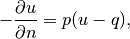
Essentially, we still stick to the model problem from
the section Multiple Dirichlet Conditions, but replace the
Neumann condition at by a Robin condition:
where  and
and  are specified functions.
The Robin condition is
most often used to model heat transfer to the surroundings and arise
naturally from Newton’s cooling law.
are specified functions.
The Robin condition is
most often used to model heat transfer to the surroundings and arise
naturally from Newton’s cooling law.
Since we have prescribed a simple solution in our model problem,
 , we adjust and such that the condition holds
at . This implies that
, we adjust and such that the condition holds
at . This implies that  and can be arbitrary
(the normal derivative at :
and can be arbitrary
(the normal derivative at :  ).
).
Now we have four parts of the boundary:  which corresponds to
the upper side ,
which corresponds to
the upper side ,  which corresponds to the lower part
,
which corresponds to the lower part
,  which corresponds to the left part , and
 which corresponds to the right part . The
complete boundary-value problem reads
which corresponds to the right part . The
complete boundary-value problem reads
The involved prescribed functions are  ,
,
 , , is arbitrary, and
  .
.
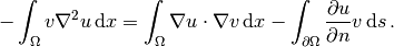
Integration by parts of 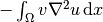 becomes
as usual
becomes
as usual
The boundary integral vanishes on  , and
we split the parts over and since we have
different conditions at those parts:
, and
we split the parts over and since we have
different conditions at those parts:

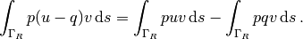
The weak form then becomes

We want to write this weak form in the standard
notation 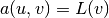 , which
requires that we identify all integrals with both
, which
requires that we identify all integrals with both  and
and  ,
and collect these in , while the remaining integrals with
and not go
into .
The integral from the Robin condition must of this reason be split in two
parts:
,
and collect these in , while the remaining integrals with
and not go
into .
The integral from the Robin condition must of this reason be split in two
parts:
We then have
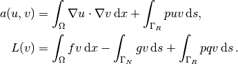
A natural starting point for implementation is the dn2_p2D.py program in the directory stationary/poisson. The new aspects are
- definition of a mesh function over the boundary,
- marking each side as a subdomain, using the mesh function,
- splitting a boundary integral into parts.
Task 1 makes use of the MeshFunction object, but contrary to the section Implementation (3), this is not a function over cells, but a function over cell facets. The topological dimension of cell facets is one lower than the cell interiors, so in a two-dimensional problem the dimension becomes 1. In general, the facet dimension is given as mesh.topology().dim()-1, which we use in the code for ease of direct reuse in other problems. The construction of a MeshFunction object to mark boundary parts now reads
boundary_parts = \
  MeshFunction("uint", mesh, mesh.topology().dim()-1)
As in the section Implementation (3) we
use a subclass of SubDomain to identify the various parts
of the mesh function. Problems with domains of more complicated geometries may
set the mesh function for marking boundaries as part of the mesh
generation.
In our case, the boundary can be marked by
class LowerRobinBoundary(SubDomain):
    def inside(self, x, on_boundary):
        tol = 1E-14   # tolerance for coordinate comparisons
        return on_boundary and abs(x[1]) < tol

Gamma_R = LowerRobinBoundary()
Gamma_R.mark(boundary_parts, 0)
The code for the boundary is similar and is seen in
dnr_p2D.py.
The Dirichlet boundaries are marked similarly, using subdomain number 2 for and 3 for :
class LeftBoundary(SubDomain):
    def inside(self, x, on_boundary):
        tol = 1E-14   # tolerance for coordinate comparisons
        return on_boundary and abs(x[0]) < tol

Gamma_0 = LeftBoundary()
Gamma_0.mark(boundary_parts, 2)

class RightBoundary(SubDomain):
    def inside(self, x, on_boundary):
        tol = 1E-14   # tolerance for coordinate comparisons
        return on_boundary and abs(x[0] - 1) < tol

Gamma_1 = RightBoundary()
Gamma_1.mark(boundary_parts, 3)
Specifying the DirichletBC objects may now make use of the mesh function (instead of a SubDomain subclass object) and an indicator for which subdomain each condition should be applied to:
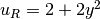
u_L = Expression('1 + 2*x[1]*x[1]')
u_R = Expression('2 + 2*x[1]*x[1]')
bcs = [DirichletBC(V, u_L, boundary_parts, 2),
       DirichletBC(V, u_R, boundary_parts, 3)]
Some functions need to be defined before we can go on with the a and L of the variational problem:
g = Expression('-4*x[1]')
q = Expression('1 + x[0]*x[0] + 2*x[1]*x[1]')
p = Constant(100)  # arbitrary function can go here
u = TrialFunction(V)
v = TestFunction(V)
f = Constant(-6.0)
The new aspect of the variational problem is the two distinct
boundary integrals.
Having a mesh function over exterior cell facets (our
boundary_parts object), where subdomains (boundary parts) are
numbered as , the special symbol ds(0)
implies integration over subdomain (part) 0, ds(1) denotes
integration over subdomain (part) 1, and so on.
The idea of multiple ds-type objects generalizes to volume
integrals too: dx(0), dx(1), etc., are used to
integrate over subdomain 0, 1, etc., inside .
The variational problem can be defined as
a = inner(grad(u), grad(v))*dx + p*u*v*ds(0)
L = f*v*dx - g*v*ds(1) + p*q*v*ds(0)
For the ds(0) and ds(1) symbols to work we must obviously connect them (or a and L) to the mesh function marking parts of the boundary. This is done by a certain keyword argument to the assemble function:
A = assemble(a, exterior_facet_domains=boundary_parts)
b = assemble(L, exterior_facet_domains=boundary_parts)
Then essential boundary conditions are enforced, and the system can be solved in the usual way:
for bc in bcs:
    bc.apply(A, b)
u = Function(V)
U = u.vector()
solve(A, U, b)
The complete code is in the dnr_p2D.py file in the stationary/poisson directory.